Quickstart

This page describes a brief tutorial on how to install and begin working with ALICA. It necessarily avoids any details on how ALICA works; instead, its focus is on helping you become acquainted with working with ALICA.

Installation

Micro-Manager 2

If Micro-Manager 2.0 or greater is not already installed on your machine, then follow the steps in this section.

1. Navigate to https://valelab4.ucsf.edu/~MM/nightlyBuilds/2.0.0-gamma/Windows/ and download the latest nightly build for your system. (Note that ALICA currently only works with Micro-Manager 2.0gamma, NOT 2.0beta.)
2. Install Micro-Manager by following the directions provided on the previously mentioned website. Make note of the installation directory, which on Windows is usually something like C:\Program Files\Micro-Manager-2.0.

ALICA

ALICA is distributed as a .jar file and is easily installed by copying the file into the Micro-Manager plugins folder.

1. Navigate to https://github.com/MStefko/ALICA/releases and download the ALICA*.jar file corresponding to the latest release.
2. Copy ALICA*.jar to the MM2ROOT/mmplugins directory, where MM2ROOT/ is the Micro-Manager installation directory.
3. Navigate to https://github.com/LEB-EPFL/ALICA_ACPack and download the ALICA_ACPack*.jar file corresponding to the latest release.
4. If you are using ALICA_ACPack version 0.2.0 or later, you will need to update a few jars that Micro-Manager uses. Download imglib2-5.3.0.jar from http://maven.imagej.net/service/local/repositories/releases/content/net/imglib2/imglib2/5.3.0/imglib2-5.3.0.jar and imglib2-roi-0.5.1.jar from http://maven.imagej.net/service/local/repositories/releases/content/net/imglib2/imglib2-roi/0.5.1/imglib2-roi-0.5.1.jar and place them in the pluginsMicro-Manager folder inside the Micro-Manager installation directory. Delete the older versions of imglib2 and imglib2-roi that are already located there.
5. Copy ALICA_ACPack*.jar to the MM2ROOT/mmplugins directory, where MM2ROOT/ is the Micro-Manager installation directory.
6. Verify that ALICA was installed and recognized by starting Micro-Manager and selecting Plugins > Device Control > ALICA in the Micro-Manager menu bar. (ALICA will not be located in the ImageJ menu bar.) The ALICA Setup window should appear, which will verify that ALICA is properly installed.

Using ALICA

ALICA reads an image stream from Micro-Manager and uses these images to estimate the real-time density of fluorescence emitting molecules within the microscope’s field of view. As the estimated density of emitting fluorophores changes (due to bleaching or changes in the sample, for example), ALICA will automatically adjust the laser power to maintain a set emitter density.

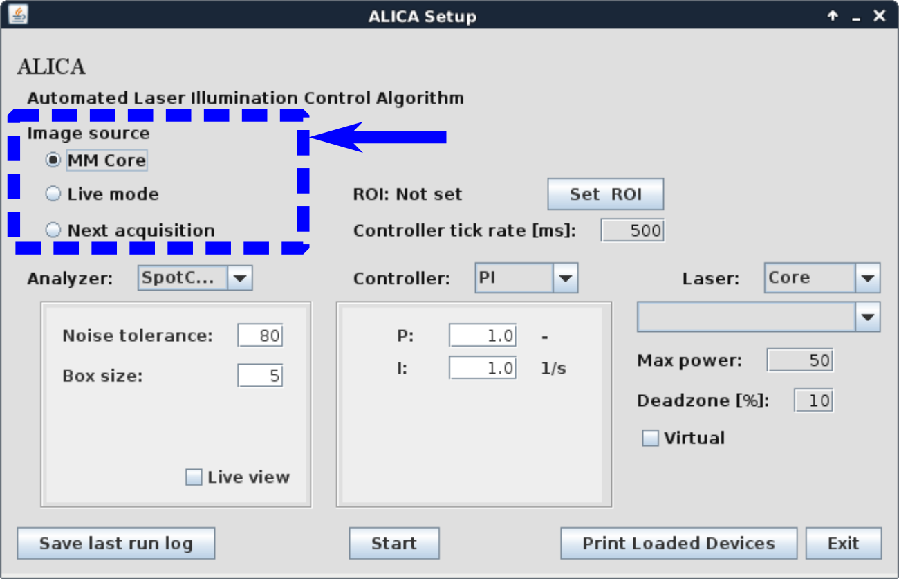
Step 1: Select an image source

First, select a source for the image stream that ALICA will analyzer. Your options include

1. the Micro-Manager core, which contains unprocessed images from the camera;
2. the Micro-Manager Live mode, which contains the images that appear in Micro-Manager’s Snap/Live View window. These images may be preprocssed by Micro-Manager’s On-The-Fly Image Processors;
3. the next Multi-Dimensional Acquisition.

We suggest choosing the Live mode option when you are just starting to use ALICA because it is the most interactive option. During actual acquisitions, MM Core is recommended due to its superior performance, unless you need to perform some image preprocessing using the MicroManager processing pipeline before feeding the images to ALICA.

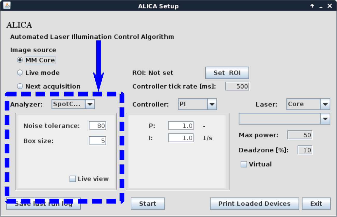
Step 2: Select and configure the analyzer

An analyzer is an algorithm that estimates the density of fluorophores that are visible in an image. At the time of this writing, ALICA included the following analyzers

1. a spot counter, which counts the number of fluorescent spots in the images;
2. AutoLase, an algorithm which estimates fluorophore densities by identifying the single pixel within the field of view that has been above a given threshold for the longest time;
3. QuickPALM, a tool which identifies fluorescent spots and then performs a subpixel localization of each spot;
4. an integrator, which simply computes the integrated intensity of an image.

The spot counter performs well for many samples and also offers a live view which provides real-time visual feedback of which spots it identifies.

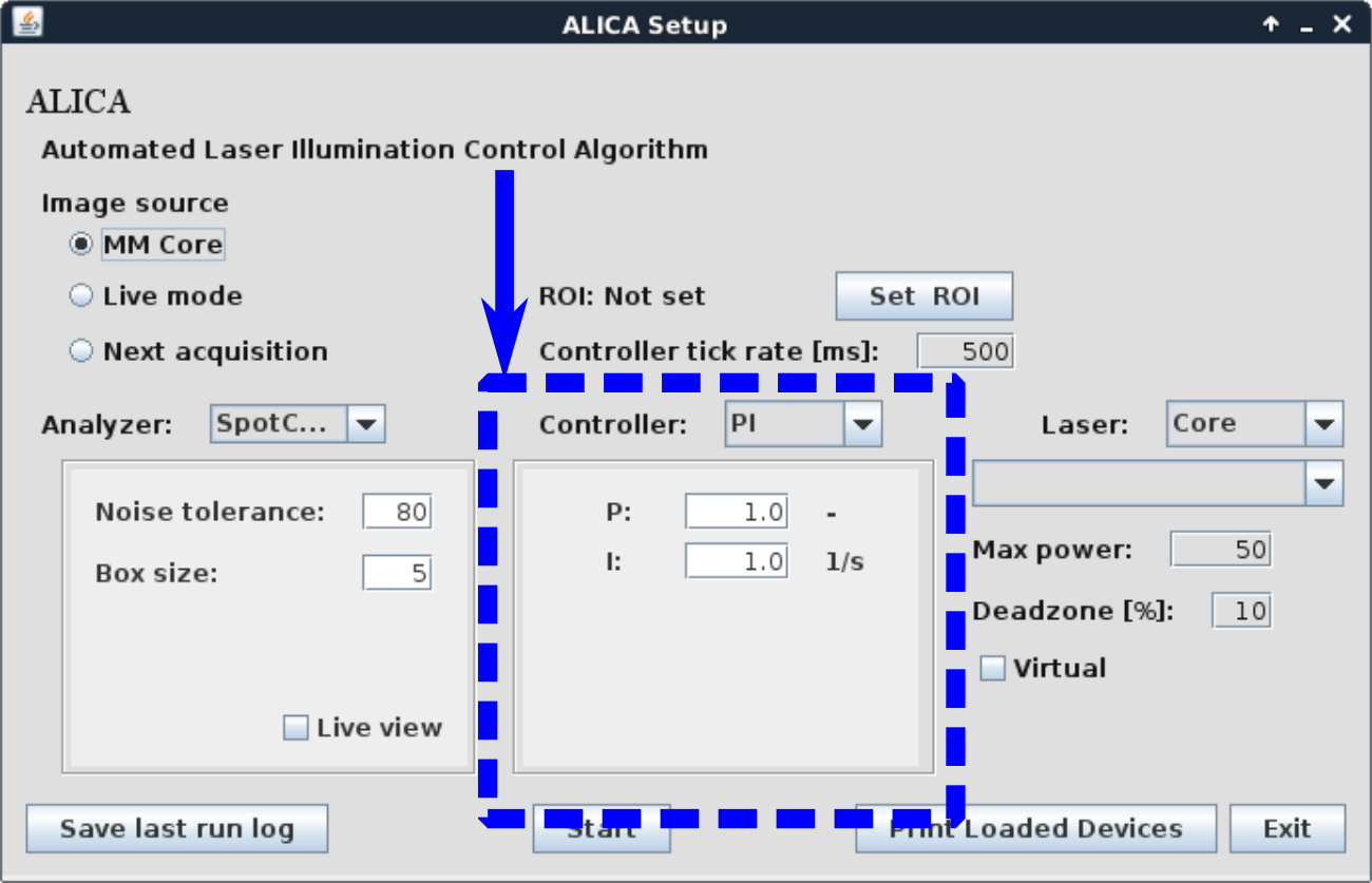
Step 3: Select and configure the controller

A controller is a feedback loop that adjusts the laser power so that the estimated density of emitters remains as close as possible to a previously determined set point. The difference between the current estimate and the set point is called the error signal. The choice of controllers includes

1. a proportional-integral (PI) controller, which responds both proportionately to the error signal and to the time integral of the error signal;
2. a manual controller, which gives control over the laser to the microscopist;
3. an inverter, which adjusts the laser by a factor that is proportional to the inverse of the error signal (e.g. high error signal > low laser power and vice versa);
4. a self-tuning (PI) controller, which uses a pulse of laser light to estimate the optimum values for the P and I parameters.

We recommend starting with manual control to first learn how the analyzer responds to changes in your sample. Once you understand a little bit about this, you can try a self-tuning PI controller. The self-tuning PI controller can only tune itself when the sample is already under STORM or PALM imaging conditions. For direct STORM, this means that the fluorophores should already be blinking.

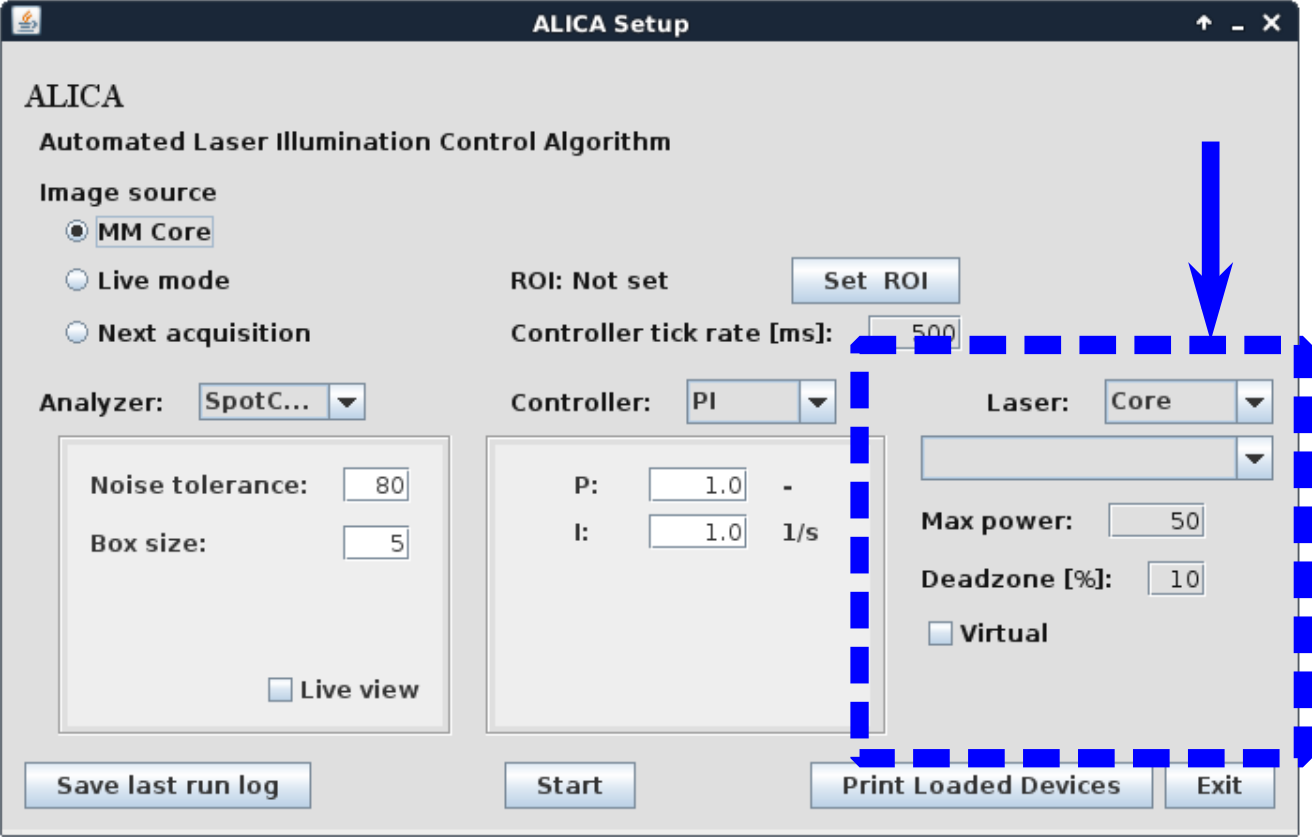
Step 4: Select the device to be controlled

A device and its property that corresponds to output power needs to be specified for the controller to actually do something. In most STORM and PALM experiments, the density of emitters is typically controlled using an ultraviolet laser. To be able select this laser, it needs to be added to the current Micro-Manager hardware configuration. Once the laser is selected, choose its power setting from the next drop-down menu.

To prevent a run-away laser illumination, you can set the maximum power for the controller. We typically do not set this above a few tens of milliWatts, but the actual value depends on the sample.

If you are testing ALICA and do not want to select a device, then check the Virtual checkbox. This will instruct the controller that it should not affect the state of any hardware devices. Checking it will allow you to test ALICA’s analyzers without performing any hardware control.

Step 5: Start the monitor

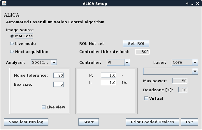
When ready, click Start in the ALICA Setup window. This will open the ALICA monitor window, which will look similar to the image below.

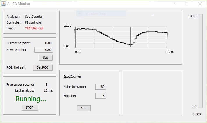
In the upper left, you can find a readout on the currently selected analyzer, controller, and laser. In this example image, the analyzer is the SpotCounter, controller is a PI controller, and the device is actually not set, i.e. the Virtual checkbox was checked in the ALICA Setup window.

Below this box you can set the desired density of fluorophores in the New setpoint: text box. After typing in a new value, click Set to activate the change. If you draw a region of interest (ROI) in the Snap/Live View window, you can set ALICA to only analyze this region by clicking the Set ROI button. You can also drag this ROI around the the Snap/Live View window in real-time and ALICA will respond in real-time.

Moving further down the left-hand side of the ALICA Monitor window, you will find information on the number of frames processed by the analyzer per second and the time taken to analyze the last frame. You may also close the ALICA Monitor window in this section by clicking the Stop button.

In the middle of the ALICA Monitor window on the top is a real-time plot of the output of the analyzer as a function of time. The units on the y-axis of this plot will depend on the output of the analyzer. For example, the SpotCounter outputs a number of spots, but AutoLase will output the longest “On” pixel in units of time.

Below this plot you may update the analyzer settings.

Finally, on the far right of the ALICA Monitor window is a status bar that reflects the current output of the laser. The maximum value of the status bar is the maximum value set in the ALICA Setup window.

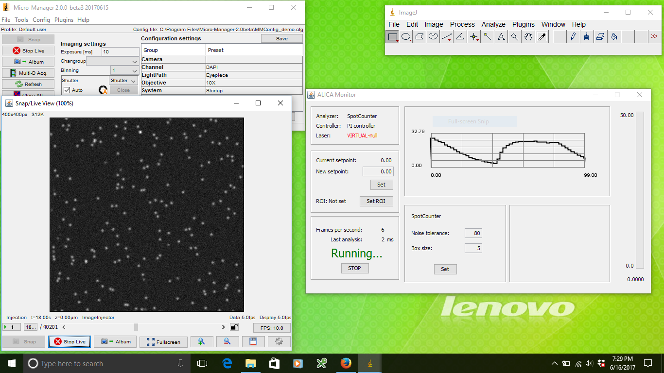
Step 6: Start taking images

When you are ready, start taking images using the source of images that you set in the ALICA Setup window. For example, if you selected Live mode, then all you need to do is start a Live stream in Micro-Manager. The different parts of the ALICA Monitor window will begin to reflect the output of the analyzer and controller once images begin arriving in this stream.

If the controller was set to Manual, try adjusting the ultraviolet laser power and watching how the output of the analyzer changes in response. If you are using a PI controller, you may notice a slight oscillation in the readout of the analyzer. This is caused by the particular values you have set for P and I.

If you selected a self-tuning PI controller, Micro-Manager will pulse the laser a short time after the acquisition has started and observe how the density of fluorophores changes in response to the pulse. It will then determine the optimum values for P and I. You may set the set point after the controller has tuned itself.

What’s next?

Tuning the parameters in ALICA may take some time and experimentation, even with the self-tuning controller. Tuning may not be easy to do on real samples due to time constraints and costly sample preparations. To ease this process, we created a simulation environment to help you learn how ALICA works.

You may read about how to setup this environment on the simulation page.